All species are of equal a priori interest
Therefore, each presence of a rare species is proportionally more
important than that of an abundant species
- To this point, we have data centered, and possibly
standardized
(depending on the weight we want to give rare vs. common species)
- We will consider the centered (but not standardized)
data:
- The next step in PCA is to fit a line through these points such
that the sum of the squares of the perpendicular distances from
the points to the line is minimized
- Axes are rotated (in this case, 127.2°)--this is called
"rigid rotation"
- New axes of the coordinate system are linear
combinations of
the axes of the original coordinate system (i.e.,
species)
- e.g., coordinate of the third quadrat on axis 1 is
(-0.605)(-1.667) + (0.796)(2) = 2.600
- (
 =
127.2°; cos =
-0.605, sin =
0.796; latter numbers are called eigenvectors--PCA is done
w/ eigenanalysis w/ real data sets)
=
127.2°; cos =
-0.605, sin =
0.796; latter numbers are called eigenvectors--PCA is done
w/ eigenanalysis w/ real data sets)
- Species are also plotted in the new coordinate
system
- Note that centering and rotating axes has not changed relative
positions of points to each other
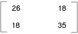
- With the centered data, total dispersion in the system is 12.667, of
which 63% was explained along species Y axis (and 37% along
species X axis)
- In the new coordinate system, the first axis accounts
for over 99% of the dispersion in the system:
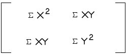
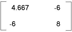
- SSCP =
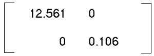
- Total dispersion = 12.561 + 0.106 = 12.667; variability
explained by first axis = 12.561/12.667 = 99.2%
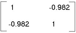
- Also, note that cross product term is 0, indicating
that new axes are orthogonal
- Whereas it required 2 axes (one of which was somewhat
less that twice as "important" as the other) to fully
describe the dispersion in the centered data, in the
new coordinate system, 99% of the dispersion in the
system is along the first axis
- This becomes very important when analyzing many
species and quadrats--w/ only 2 species, it is not
necessary to conduct a PCA (because gradient can
be interpreted directly)
- Summary of PCA algorithm:
- Species are "plotted" in quadrat-dimensional space
- Data are centered, and possibly standardized
- A "best-fit" line is projected through the data (PCA axis 1)
- Another line is fit through the data, orthogonal to the
first (PCA axis 2)
- and so on, for up to n-1 axes (where n=number of
quadrats)
Original axes vs. PCA axes:
- Arrangement of points never changes; only the axes change
(standardizing changes arrangement of points)
- Angular relations between points as viewed from the original
are unaltered by the second transformation (rigid rotation),
but they are changed by the first transformation (centering)
- Original axes have a simple meaning: abundances of
individual species. PCA axes have a complex meaning:
linear combinations of abundances {sum of the abundance
times the eigenvector (sine or cosine of the angle) for each
species}.
- PCA axes concentrate variance or structure of the point
configuration into relatively few axes, in contrast to the
high dimensionality of the original data.
Note that PCA involves analysis of community data alone--
environmental data are not included. Thus, environmental
interpretation of PCA results is a separate step.
Previous
lectureNext
lecture

 X=8
X=8 
 =
= 
 ÷ (3-1) =
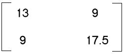
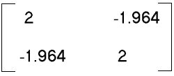 --> SSCP/(n-1) =