Special issue: Selected papers from the IALC Conference:
Assessing Capabilities of Soil and Water Resources in Drylands:
The Role of Information Retrieval and Dissemination Technologies

Special issue: Selected papers from the IALC Conference: Assessing Capabilities of Soil and Water Resources in Drylands: The Role of Information Retrieval and Dissemination Technologies |
|
by D.W. Johnson, R.B. Susfalk, W.W. Miller, J.M. Murphy, D.E. Todd, P. Verburg and R.F. Walker
| "For quantification of carbon and nutrient pools (kg/ha) in arid environments, completely random sampling is recommended. ...In general, it is recommended that mineral soils be sampled by depth after determining the nominal depths corresponding to major horizons. " |
Introduction(Back to top) The presence of islands of fertility in arid soils presents significant sampling problems when calculating soil pool sizes (i.e., kg/ha or g/m2) of organic matter and nutrients which are not addressed by the semi-variogram approach and are not easily solved by soil sampling protocols typical of more mesic systems. Characterization of pool sizes of soil C in particular is rapidly becoming a necessity in view of the potential role of soils in the global C cycle. Even a cursory review of published global carbon budgets reveals that soils could be either a major source or sink for carbon. Schimel (1995) estimated that soils contain approximately twice as much C (1580 x 1015g) as the atmosphere (750 x 1015g) or terrestrial vegetation (610 x 1015g). Less than 1% of the terrestrial C reservoir (1.9 x 10¹⁵g C/yr) is emitted to the atmosphere through changing land use each year, whereas amounts of C entering soil as detritus (61.4 x 10¹⁵g C/yr) and leaving by respiration (60 x 1015g C/yr) are far greater (Schimel 1995). In light of these observations, reliable information is needed on soil C pool sizes as well as the effects of management practices on these pools. The latter will require measuring changes in soil C pools, a task that is challenging even in relatively uniform soils and especially daunting in arid soils with their inherent spatial variability. Many detailed reviews and analyses have been written on the nature of arid soils and the important role of fertility islands in them (West 1991; Charley and Wext,1975; Tiedemann and Klemmedson 1973, 1986; Halvorson et al. 1994, 1997; Klemmedson and Tiedemann 1986; Virginia and Jarrell 1983; Everett et al. 1986; Schlesinger et al. 1996). The reader is referred to these references for more detail about this subject. What is often lacking, however, is a full discussion of the inherent problems encountered in sampling soils in the field and an analysis of potential solutions to these problems. Thus, the primary purpose of this paper is to review sampling and characterization problems in arid soils and potential solutions to them. Sampling litter and soils in a spatially heterogeneous environment(Back to top) Peterson and Calvin (1986) note that there are three sources of error in soil sampling:
Although the authors do not so state, we believe that sampling error and especially selection error are generally much more important than measurement error in sampling of non-agricultural soils. Peterson and Calvin (1986) also discuss the advantages and disadvantages three methods of sampling in the horizontal scale: simple random sampling, stratified random sampling, and systematic sampling (i.e., a regular grid with established sampling points). Their review of the literature indicated that systematic sampling is the preferred method in nearly all cases where the three methods have been compared. They note, however, that exceptions occur where the variation is periodic, such as where there are rows of crops, and in cases where there is a fertility gradient along rows of a field. They also note that one of the major problems with systematic sampling is the estimation of sampling error from the sample itself, and they offer three alternative methods:
We have concluded that neither stratified nor systematic sampling is appropriate for soils in semi-arid forests of the Sierra Nevada Mountains. Stratified sampling was rejected because the boundaries of the strata (the borders between the islands of fertility and interspaces) are diffuse, leading to arbitrary and inconsistent delineations of strata boundaries among individual investigators and between sites and over time. We judged that the definitions of strata boundaries were sufficiently unclear and inconsistent as to overwhelm any possible advantage to stratification when sampling either soils or litter for the purposes of measuring pools sizes. Systematic sampling is judged inappropriate for several reasons. First of all, the population of samples is not random but varies systematically, both over the landscape as a whole and within strata (e.g., within the islands of fertility), thus violating the premises of alternatives 1 and 2 above for defining sample variability. Alternative 3 is considered to be too expensive in time, labor, and analytical costs for most cases. We find is most convenient to plot random coordinates on a Cartesian system and then convert these to polar coordinate so that random sampling points can be easily determined in the field from distance and azimuth measurements from the plot center. When sampling for the purpose of determining pool sizes, we avoid selection error if at all possible. If a sample point lies directly beneath a tree, it must be discarded; however, if a sample point lands on a large boulder, it is included: the fine earth fraction is 0, and the bulk density is defined as mineral density (2.65 g/cm3 or a density determined from rock samples taken nearby). Accounting for vertical variation: Soil horizons |
|
|
A fundamental feature of soils is horizonation, and this must be taken into account when sampling soils, either for pool sizes or for chemical concentrations. The first and usually most distinct soil horizons are the organic (O) horizons, which consist of organic matter. The three major organic horizons are Oi, consisting of slightly decomposed plant litter, Oe, moderately decomposed plant litter (still recognizable as to species), and Oa, highly decomposed organic matter (not recognizable as to species). The distinctions between these horizons are often arbitrary and therefore will vary with investigator and field conditions such as moisture (Federer 1982). Furthermore, separation of the Oa horizons from underlying A horizons (mineral soils high in organic matter) can be very difficult: soil particles and even rocks can be intermingled with Oa horizons and are invariably included in Oa samples. In the case of small particles, this can be corrected for by determining ash content (combustion); in the case of rocks and larger particles, it is often necessary to separate the organic from mineral phase by floating. Unfortunately, soil profiles are in actuality continuous chromatographs; the definitions of horizons and boundaries are often arbitrary and the boundaries between are often indistinct. Figure 1 illustrates a typical distribution of soil organic matter concentration with depth in a given profile. When sampling for pool sizes, it is important to sample horizons proportionately, that is, to take samples from each horizon within a constant horizontal area, as in a core, so as not to bias the samples with more or less of one depth or another within the horizon. Thus, if soil samples are to be taken by shovel or trowel, it is important to keep the sampling hole proportional and avoid the natural tendency to narrow the hole area with depth, as illustrated by the biased sample in Figure 1. |
|
|
To complicate matters further, horizon depths are often quite variable in the horizontal direction, especially in disturbed landscapes. Figure 2 illustrates this, and the sampling problems that could be encountered if soils are sampled by depth rather than by horizon. A constant depth of sampling will not include all of the A horizon in sample points where the horizon is thick and will include some amount of the underlying horizon in sample points where the horizon is thin. It would seem ideal, then, to sample soils by horizon rather than by depth at each sampling point. Unfortunately, this is only possible if pits are dug at each sampling point or in the event that the soil is very friable and free of stones so that an open-faced punch auger can be used to determine depths while coring. In the event that pits are dug, the possibilities for resampling in the future near the same location are greatly diminished. In practice, the usual procedure is to dig a pit in the general area of the sampling to determine the nominal depths of the major horizons and use that to establish sampling depths to be used subsequently with a coring device. Thus, the sampling problems illustrated in Figure 2 are often a major factor in soil variability on the horizontal scale. A further problem may occur in soils subject to expansion and contraction (i.e., those containing smectite clays or those which accumulate or lose considerable amounts of organic matter). If it is desired to measure changes in soil properties over time in such cases (as will be the case for soil C sequestration), the shrinking and swelling of soils will cause changes in horizon depths that must be taken into account. Such changes can be calculated if bulk density is measured at each sampling date. Although it is generally preferable to sample soils by horizon, it is often the case that samples must be taken to a constant lowest depth, unless total soil depth is dictated by the presence of bedrock. This is because soil depth is one of the major variables affecting total soil mass and therefore total soil pools of a given nutrient. Even in the cases of soil C and N, where the highest concentrations occur in surface horizons, total depth of soil considered is often a major factor in total soil pools because deeper horizons are often more dense and make up considerable mass. Estimating soil mass Obtaining representative soil element concentrations over the landscape and by horizon is adequate for some purposes (relating to plant fertilizer needs or water quality only), but it is less than half of the battle in terms of estimating soil nutrient pool sizes. Measurements of soil mass are all fraught with sampling problems and errors, and can be far more tedious than taking samples for chemical analysis. Three fundamental things are needed in order to obtain estimates of soil mass: bulk density of the soil, percent coarse fragments (mineral material, rocks, stones, boulders greater than 2 mm diameter), and depth. Bulk density can be measured using various methods (clod, core, excavation, and radiation) which are fully reviewed by Blake and Hartge (1986). These methods have been developed largely for agricultural soils which are low in large coarse fragments; wildland soils in forests and arid lands often contain substantial amounts of large coarse fragments, but these are seldom measured accurately because of the difficulties involved. Indeed, large coarse fragments are often simply estimated by eye or from very sparse and general data sets, and then liberally used in detailed calculations of soil C and nutrient content. We feel that improper and inaccurate measurements of large coarse fragments is the major source of error in estimation of soil C and nutrient pools in many wildland soils. Measurements of large coarse fragments are usually made by excavation methods and are difficult, time consuming, and destructive to the site being sampled. Hamburg (1984) outlined a quantitative pit procedure for measurement of bulk density and large coarse fragments in very stony soils in Hubbard Brook, New Hampshire. The method involves digging a very straight-walled pit, 1 m2 in area, and removing and weighing all material from it, by horizon. The volume of the hole is then estimated by using a template which subdivides the area into a 25-cell grid and measuring the perpendicular distance to the soil surface at each grid point. Problems were encountered with large boulders protruding from the pit walls, and their volume and mass had to be measured separately. Bulk density of the soil fraction was then estimated by coring in the pit walls. Case studies of soil sampling in semi-arid forests(Back to top) |
|
|
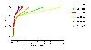
A case study of the results of litter and soil sampling in a semi-arid forest in the eastern Sierra Nevada Mountains (Little Valley, Nevada) is shown in Figure 3 (Johnson et al. 1997; Susfalk, 2000). The study site is at an elevation of 2015 m, with a slope of less than 3% and with an overstory vegetation dominated by widely-spaced 110-120-year-old lodgepole pine (Pinus contorta Dougl.) with occasional Jeffrey pine (Pinus jeffreyii [Grev. and Balf.]). Understory vegetation consists of bitterbrush (Purshia tridentata D.C.), and various grasses and forbs. Soils at the study site are the Marla soil series, sandy, mixed Aquic Cryumbrepts derived from colluvium of decomposed granite. The site is characterized by pronounced islands of fertility associated with the overstory trees. Sampling points were established in a completely random fashion and both litter and soils were sampled by horizon rather than depth using large sample pits (Johnson et al. 1997; Susfalk, 2000). The depth of sampling for the A horizons varied from 3 to 10 cm, the depths for the B horizons varied from 20 to 22 cm, and BC horizons were all sampled to 50 cm. In pits 1 through 4, we were able to get samples below 50 cm and determined that the soil was at least 1 m deep. Figure 3A shows that C concentrations vary most in the surface horizons, and Figure 3B shows the depth distribution of C content (kg/ha) for each individual pit. In Figure 3B, total O horizon C content is shown above the 0 line and soil C contents by horizon (as negative numbers) below the 0 line. The first, second, third, and (where present) fourth bars below the 0 line in Figure 3B represent the C contents in the A, B, BC, and C horizons, respectively, and are coded so that the depth of sampling is indicted. |
|
|
The island of fertility effect is clearly shown here, with extreme variability in O and A horizon C contents. However, the relationship between O horizon C content (the best index of inputs via litterfall) and soil C concentrations or content is not straightforward. It clear that pit 4 had the greatest C contents in both O horizons and mineral soils as well as the greatest A horizon C concentration, but A horizon depth was among the lowest. Also, there were no statistically significant correlations between O horizon C content and A horizon C concentration, A horizon C content or A horizon depth. Nor were there any significant correlations in C concentrations between A and B, B and BC, or BC and C horizons. It is generally assumed that most soil C is contained in the A horizon. In this site, O horizon C contents rival those in the mineral soil (to a depth of 50 cm) in some cases, however (pits 4 and 6). In some cases, total soil C content is dominated by the A horizon: A horizon C content accounts for half or more of total soil C in pits 4, 5, and 6. In other cases, however, (pits 1, 2, and 3), the C contents of the lower horizons are relatively important even though the concentrations are very low. Where the data is available (pits 1 through 4), it is clear that the C content of the C horizon (50-100 cm depth) contributes significantly (20 to 33%) to the total soil C content even if concentrations in that horizon are low. This is because of the large mass of the soil in the C horizon, which is a result mostly of its thickness. Coarse fragment (> 2 mm) contents are low in this particular soil (< 3%), but coarse fragment content has a substantial effect on soil C pools in stonier soils. The subject of coarse fragments and their measurement is discussed in more detail below. Truckee, California We used a variation on the quantitative pit method of Hamburg (1984) to sample stony soils in the eastern Sierra Nevada Mountains. The site is dominated by Jeffrey pine in the overstory and has a somewhat sparse understory consisting of bitterbrush, occasional manzanita (Arcostaphylos patula Greene), snowbush (Ceanothus velutinus Dougl.), and squawcarpet (Ceanothus prostratus). Soils are the Kyburz series, fine-loamy, mixed, frigid Ultic Haploxeralfs derived from andesite. In our variation of the Hamburg (1984) method, the volume of the hole is not measured directly, but calculated from the mass and density of the soil, stones, and woody material removed from the pits. Unlike Hamburg (1984) who established plots arbitrarily away from large boulders and trees, we established pits in a simple random fashion over a series of 24 plots covering three landscape positions: upper and lower slope in one location (which had been thinned and later received prescribed fire) and another location which had never been thinned but later received prescribed fire. We also measured litter and coarse woody debris mass on each plot. |
|
|
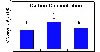
The results show considerable amounts of coarse fragments (which were classified mainly as cobbles, being rocks 7.5 to 25 cm diameter) within all soils (Figure 4). The US classification system calls for a mention of coarse fragments if they constitute over 15% of the whole soil volume. If rock fragments constitute over 35% in the control section (soil from the top of the Bt horizon down to a depth of 50 cm), the term skeletal is used in the particle size descriptor. Thus, the soil in this site may be classified as cobbly in all cases and in the case of location 1, upslope, it would be cobbly, loamy-skeletal, mixed, frigid Ultic Haploxeralf. The system also calls for the word "very" to precede the cobbly adjective in cases where coarse fragments constitute 35 to 60% by volume, and the upslope set of plots in location 1 nearly qualify for that. Perhaps most important, the carbon concentrations in these soils differ significantly from one another, the rock fragment contents in these soils differ significantly from one another, and yet the carbon contents do not differ significantly because the variations in carbon concentration are offset by those in rock fragments (Figure 4). This example illustrates the importance of obtaining accurate measurements of rock fragments when estimating soil C pools, and this cannot be made without tedious and time-consuming measurements. Conclusions(Back to top) References(Back to top) Burke, I.C., W.A. Reiners, D.L. Sturges, and P.A. Matson. 1987. Herbicide treatment effects on properties of mountain big sagebrush soils after fourteen years. Soil Science Society of America Journal 51: 1337-1343. Charley, J.L., and N.E. West. 1975. Plant-induced soil chemical patterns in some shrub-dominated semi-desert ecosystems of Utah. Journal of Ecology 63: 945-963. Everett, R., S. Sharrow, and D. Thran. 1986. Soil nutrient distribution under and adjacent to singleleaf pinyon crowns. Soil Science Society of America Journal 50: 788-792. Federer, C.A. 1982. Subjectivity in separation of organic horizons of the forest floor. Soil Science Society of America Journal 46: 1090-1093. Garner, W., and Y. Steinberger. 1989. A proposed mechanism for the formation of "Fertile islands" in the desert ecosystem. Journal of Arid Environments 16: 257-262. Halvorson, J.J., J. Bolton, Jr, and J.L. Smith. 1997. The pattern of soil variables related to Artemesia tridentata in a burned shrub-steppe. Soil Science Society of America Journal 61: 287-294. Halvorson, J.J., J. Bolton, Jr, J.L. Smith, and R.E. Rossi. 1994. Geostatistical analysis of resource islands under Artemesia tridentata in the shrub-steppe. Great Basin Naturalist 54: 313-328. Hamburg, S.P. 1984. Effects of forest growth on soil nitrogen and organic matter pools following release from subsistence farming. In Forest Soils and Treatment Impacts, Proceedings of the Sixth North American Forest Soils Conference, ed. E.L. Stone, 135-158. Knoxville, Tennessee: University of Tennessee. Klemmedson, J.O., and A.R. Tiedeman. 1986. Long-term effects of mesquite removal on soil characteristics: II. Nutrient availability. Soil Science Society of America Journal 50: 476-480. Peterson, R.G., and L.D. Calvin. 1986. Sampling. 33-52 In Methods of soil analysis. Part 1. Physical and mineralogical methods, ed. A. Klute, 33-52. Second ed. Agronomy Series No. 9. Madison, Wisconsin: Soil Science Society of America. Rossi, R.E., D.J. Mulla, A.G. Journel, and E.H. Franz. 1992. Geostatistical tools for modeling and interpreting spatial dependence. Ecological Monographs 62: 277-314. Schlesinger, W.H., and A. Pilmanis. 1998. Plant-soil interactions in deserts. Biogeochemistry 42: 169-187. Schlesinger, W.H., J.A. Raikes, and A.F. Cross. 1996. On the spatial pattern of soil nutrients in desert ecosystems. Ecology 77: 364-374. Schlesinger, W.H., J.F. Reynolds, G.L. Cunningham, L.F. Huenneke, W.M. Jarrell, R.A. Virginia, and W.G. Whitford. 1990. Biological feedbacks in global desertification. Science 247: 1043-1048. Tiedemann, A.R., and J.O. Klemmedson. 1973.Nutrient availability in desert grassland soils under Mesquite (Prosopis juliflora) trees and adjacent open areas. Soil Science Society of America Journal 37: 107-111. Tiedemann, A.R., and J.O. Klemmedson. 1986. Long-term effects of mesquite removal on soil characteristics: I. Nutrients and bulk density. Soil Science Society of America Journal 50: 472-475. Virginia, R.A., and W.M. Jarrell. 1983. Soil properties in a mesquite-dominated Sonoran desert ecosystem. Soil Science Society of America Journal 47: 138-144. West, N.E. 1991. Nutrient cycling in soils of semiarid and arid regions. In Semiarid lands and deserts: Soil resource and reclamation, ed. J. Skujins, 295-332. New York: Marcel Dekker. Wilkeem, S.J., and M.D. Pitt. 1982. Soil nitrogen gradients as influenced by sagebrush in southern British Columbia. Northwest Science 56: 276-286. |
|
|
![]()
(Back to top)
D.W. Johnson, Environmental and Resource Sciences, University of Nevada, Reno;
Reno, Nevada 89557
R.B. Susfalk, Environmental Sciences Division, Oak Ridge National Laboratory, Oak Ridge, Tennessee 37830
W.W. Miller, Environmental and Resource Sciences, University of Nevada, Reno; Reno, Nevada 89557
J.M. Murphy, Environmental and Resource Sciences, University of Nevada, Reno; Reno, Nevada 89557
D.E. Todd, Jr, Environmental Sciences Division, Oak Ridge National Laboratory, Oak Ridge, Tennessee 37830
P. Verburg, Division of Earth and Environmental Research, Desert Research Institute, Reno, Nevada 89512
R.F. Walker, Environmental and Resource Sciences, University of Nevada, Reno; Reno, Nevada 89557
About the Arid Lands Newsletter